42 excel chart remove 0 data labels
Apache OpenOffice Community Forum - [Solved] Creating a Timeline with ... There does seem to be one glitch that I don't understand: if I open Hagar's sample .ods, activate the first chart, that shows the number labels, and do... 1) Right-click on a data label > Format Data Labels > Data Labels ___ Show value as a number: NO ___ Show category: YES ___ OK (labels disappear) 2) Right-click anywhere > Data Ranges > Data ... How to create graphs in Illustrator - Adobe Inc. If you accidentally enter graph data backward (that is, in rows instead of columns, or vice versa), click the Transpose button ( ) to switch the columns and rows of data. To switch the x and y axes of scatter graphs, click the Switch X/Y button ( ) . Click the Apply button or press the Enter key on the numeric keypad to regenerate the graph.
How to make a 3 Axis Graph using Excel? - GeeksforGeeks A Format Data Series dialogue box appears. In the series Option, select the blue line as the Secondary Axis . Step 6: Now, you need to remove the Chart Title of graph1. Double click on the chart title of graph1. Format Chart Title dialogue box appears. Go to Text options. In the Text Fill, select No Fill.

Excel chart remove 0 data labels
Questions from Tableau Training: Can I Move Mark Labels? Option 1: Label Button Alignment. In the below example, a bar chart is labeled at the rightmost edge of each bar. Navigating to the Label button reveals that Tableau has defaulted the alignment to automatic. However, by clicking the drop-down menu, we have the option to choose our mark alignment. Create an Excel Dashboard from Scratch in 8 Steps (or Just 3 with Databox) Firstly, press 'Select Data' after right-clicking the chart. Choose the 'Add in Legend Entries' option. You can choose the title of the columns in the 'Series name' field, and the data in the 'Series values' field. In most cases, the X-axis won't be labeled properly. You can fix this by going to the 'Horizontal Axis Labels' tab and clicking 'Edit'. Understand charts: Underlying data and chart representation (model ... Charts in model-driven apps can be further classified into the following: Single-series charts: Charts that display data with a series (y) value mapped to a category (x) value. Multi-series charts: Charts that display data with multiple series values mapped to a single category value. Multi-series charts include stacked column charts, which ...
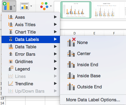
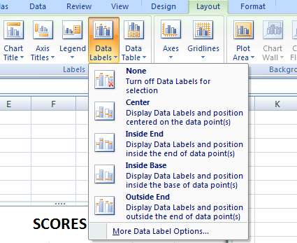
Excel chart remove 0 data labels. How to Use Excel Pivot Table Date Range Filter- Steps, Video The column heading says "Row Labels". To choose the pivot field that you want to filter, follow these steps: In the pivot table, click the drop down arrow on the Row Labels heading. In the Select Field box, slick the drop down arrow. Select the date field that you want to filter. A Step-by-Step Guide on How to Make a Graph in Excel Using this, you can find all the zeros and remove them. You can also replace all the formula references. Remove Extra Spaces You can get rid of unwanted spaces between words or numbers which aren't visible using the TRIM function. The syntax is: =TRIM (text) This function takes input as text and eliminates extra spaces. support.microsoft.com › en-us › officeAdd or remove data labels in a chart - support.microsoft.com You can add data labels to show the data point values from the Excel sheet in the chart. This step applies to Word for Mac only: On the View menu, click Print Layout . Click the chart, and then click the Chart Design tab. Excel Formula Symbols Cheat Sheet (13 Cool Tips) - ExcelDemy The formula for calculating the Area is, =A2*B2. Now place this formula in cell C2 and press enter. If you select this cell C2 again you will see a green-colored box surrounds it, this box is known as the fill handle. Now drag this fill handle box downwards to paste the formula for the entire column.
Excel Pivot Tables - by contextures.com When you set up a pivot table, and put fields into the Rows Area or Columns area, Excel groups the items, and calculates the totals for each group. For example, see count of products for each Unit Price. Each item should only be listed once in the pivot table, but sometimes you might see duplicates. Continue reading. Create Excel Waterfall Chart Template - Download Free Template Select the Horizontal axis, right-click and go to Select Data. Select cell C5 to C11 as the Horizontal axis labels. Right-click on the horizontal axis and select Format Axis. Under Axis Options -> Labels, choose Low for the Label Position. Change Chart Title to "Free Cash Flow.". Remove gridlines and chart borders to clean up the waterfall ... Is there a way to move axis labels farther from excel graph area? 1 1 Right-click on the labels and choose "Format Axis" from the dropdown menu, under Labels, increase "Distance from Axis" - cybernetic.nomad May 27 at 21:04 Add a comment Browse other questions tagged excel graph or ask your own question. Extract a unique distinct list and ignore blanks - Get Digital Help Copy cell B2 and paste to cells below. Back to top. 1.1 Explaining the LOOKUP formula in cell D3 Step 1 - Check cell range B3:B12 for non-empty cells. If a cell contains a value TRUE is returned. The following line is a logical expression, cells not equal to nothing return TRUE.The less and larger than characters are logical operators that evaluates to boolean values, True or False.
Clear a Chart or Graph in LabVIEW - NI Graph. You can clear a graph programmatically by writing an empty array to its Value property: Make sure the graph is clear by right-clicking the graph and choosing Data Operations>>Clear Graph. Right-click the graph and select Create>>Property Node>>Value. Right-click Value and select Change to Write. Right-click the Value Terminal and select ... Mathcad Ideas - PTC Community Symbolic Mathcad Engine. Status: New Idea Submitted by RW_8551085 on 06-06-2022 03:09 PM. Comment. I am running Mathcad Prime 6.0.0., but this still occurs in Mathcad Prime 8. I am trying to use the symbolic engine to output a symbolic equation. In this example the equation has 6 constants and 1 variable. The output doesn't combine all of ... › documents › excelHow to create progress bar chart in Excel? - ExtendOffice Then close the Format Data Series pane, and then click to select the whole chart, and click Design > Add Chart Element > Data Labels > Inside Base, all data labels have been inserted into the chart as following screenshot shown: 5. And then you should delete other data labels and only keep the current data labels as following screenshot shown: 6. › gantt-chart › how-to-makeExcel Gantt Chart Tutorial + Free Template + Export to PPT Right-click the white chart space and click Select Data to bring up Excel's Select Data Source window. On the left side of Excel's Data Source window, you will see a table named Legend Entries (Series). Click on the Add button to bring up Excel's Edit Series window where you will begin adding the task data to your Gantt chart.
How to Add Data Labels to your Excel Chart in Excel 2013 - YouTube
A Solution to Tableau Line Charts with Missing Data Points Yes! The obvious answer is to use the IFNULL function, and this would work great if our data looked like this: But our data doesn't look like this, so the IFNULL function won't work as there are no nulls in the data. As mentioned above, we don't have null values, we have no data. This is a critical and often misunderstood point. The Solution
How to Make Charts and Graphs in Excel | Smartsheet
Excel FAQ - Application and Files Press the Shift key, and click the X at the top right of one of the Excel windows. You will be prompted to save any unsaved files, and then all the windows will close. 3. Press the Alt key, and tap the F key, then tap the X key. When you press Alt+F, the File tab is activated.
how to make a excel graph.
Excel Slicer And Timeline - Tutorial With Examples How To Create Timeline In Excel. Click anywhere on the Pivot table, and the PivotTable Tools ribbon will be displayed. Go to PivotTable Tools -> Analyze -> Insert Timelines. Click on Insert Timeline. Insert Timeline dialog which will only show the date column of your table will appear. Select the date checkbox.
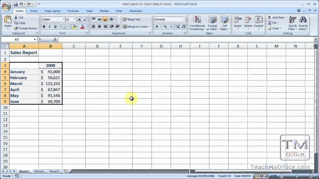
Add Labels to Chart Data in Excel - YouTube
support.microsoft.com › en-us › officeInsert a chart from an Excel spreadsheet into Word Keep Source Formatting & Link Data. Keeps the Excel theme. Keeps the chart linked to the original workbook. To update the chart automatically, change the data in the original workbook. You also can select Chart Tools> Design > Refresh Data. Picture. Becomes a picture. You can’t update the data or edit the chart, but you can adjust the chart ...

Excel/R (?) Pie Chart with Subsections - Super User
linkedin-skill-assessments-quizzes/microsoft-excel-quiz.md at ... - GitHub A cell contains the value 7.877 and you want it to display as 7.9. How can you accomplish this? Use the ROUND () function. Click the Decrease Decimal button twice. In the cells group on the Home tab, click Format > Format Cells. Then click the Alignment tab and select Right Indent. Click the Decrease Decimal button once. Q13.

Microsoft Excel Tutorials: The Chart Layout Panels
A Beginner's Guide on How to Plot a Graph in Excel In Excel, you have huge ranges of choice for charts and graphs to create. This includes column chart, line chart, pie chart, area chart, scatter plot, (Stock, Surface, Radar, Bubble Doughnut etc.) charts. Obviously, you can choose any chart and graph as you desire. STEP 5: Select your data table and insert your desired graph

How to Add Data Labels in Excel - Excelchat | Excelchat
› combination-clustered-andCombination Clustered and Stacked Column Chart in Excel Click the Secondary Axis labels and press delete to remove it. We still have some extra chart lines corresponding to the “Total”, the “Primary Scale”, and the “Secondary Scale”. Starting with the “Total” line, click the data series in the chart. In the Format ribbon, click Format Selection. On the Fill & Line options, select No ...

Elements of an Excel Chart | ExcelDemy.com
50 Excel Shortcuts That You Should Know in 2022 - Simplilearn First, let's create a pivot table using a sales dataset. In the image below you can see that we have a pivot table to summarize the total sales for each subcategory of the product under each category. Fig: Pivot table using sales data The image below depicts that we have grouped the sales of bookcases and chairs subcategories into Group 1.

Excel Graph - 2 Line chart / Each line representing it's own data set - Stack Overflow
› documents › excelHow to group (two-level) axis labels in a chart in Excel? The Pivot Chart tool is so powerful that it can help you to create a chart with one kind of labels grouped by another kind of labels in a two-lever axis easily in Excel. You can do as follows: 1. Create a Pivot Chart with selecting the source data, and: (1) In Excel 2007 and 2010, clicking the PivotTable > PivotChart in the Tables group on the ...

Excel Charts | Waterfall, Funnel and Pareto Charts
How to remove text or character from cell in Excel - Ablebits.com Select a range of cells where you want to remove a specific character. Press Ctrl + H to open the Find and Replace dialog. In the Find what box, type the character. Leave the Replace with box empty. Click Replace all. As an example, here's how you can delete the # symbol from cells A2 through A6.

Do My Excel Blog: How to hide the zero percent labels in an Excel pie chart
Gridlines in Excel - Overview, How To Remove, How to Change Color How to Remove Excel Gridlines The easiest way to remove gridlines in Excel is to use the Page Layout tab. Click the Page Layout tab to expand the page layout commands and then go to the Gridlines section. Below Gridlines, uncheck the view box. The keyboard shortcut option to remove the gridlines is to press Alt and enter W, V, G.
Excel Charts: Positive/Negative Axis Labels on a Bar Chart
How to add a single vertical bar to a Microsoft Excel line chart In the Chart Layouts group, click Add Chart Element. From the dropdown, choose Axes. From the resulting submenu, choose Secondary Vertical ( Figure J ), which displays the axes values to the right...

34 Label Chart In Excel - Labels Database 2020
Two level axis in Excel chart not showing • AuditExcel.co.za In order to always see the second level, you need to tell Excel to always show all the items in the first level. You can easily do this by: Right clicking on the horizontal access and choosing Format Axis. Choose the Axis options (little column chart symbol) Click on the Labels dropdown. Change the 'Specify Interval Unit' to 1.

Microsoft Excel Tutorials: The Chart Layout Panels
How to Remove Table Formatting in Excel (2 Smart Ways) Let`s see how the thing is done. First, select the entire table. After this press on to the Home tab and in the Editing section of Home tab look for the Clear option. After selecting the Clear option, you will get a drop-down list. From there, select the Clear Formats option.

Bar Chart No Labels - Free Table Bar Chart
Slicer not working on Chart in VBA, but works after selecting chart ... 'create a new chart sheet and place it at the beginning of the destination workbook Dim oChartSheet As Chart ' Set oChartSheet = destinationWorkbook.Charts.Add (destinationWorkbook.Sheets (1)) Set oChartSheet = wS.Shapes.AddChart.Chart 'set the properties for the chart With oChartSheet .SetSourceData Source:=sourceDataRange1
Excel Charts: Polar Plot Chart. Polar Plot Created Using Radar Chart
› dynamically-labelDynamically Label Excel Chart Series Lines • My Online ... Sep 26, 2017 · Hi Mynda – thanks for all your columns. You can use the Quick Layout function in Excel (Design tab of the chart) to do the labels to the right of the lines in the chart. Use Quick Layout 6. You may need to swap the columns and rows in your data for it to show. Then you simply modify the labels to show only the series name.

How to Add Data Labels to an Excel 2010 Chart - dummies
Publish and apply retention labels - Microsoft Purview (compliance) Solutions > Records management > > Label policies tab > Publish labels If you are using data lifecycle management: Solutions > Data lifeycle management > Label policies tab > Publish labels Don't immediately see your solution in the navigation pane? First select Show all. Follow the prompts to create the retention label policy.

How to get Excel Chart Columns with no gaps • AuditExcel.co.za
Understand charts: Underlying data and chart representation (model ... Charts in model-driven apps can be further classified into the following: Single-series charts: Charts that display data with a series (y) value mapped to a category (x) value. Multi-series charts: Charts that display data with multiple series values mapped to a single category value. Multi-series charts include stacked column charts, which ...
Post a Comment for "42 excel chart remove 0 data labels"